1. Basic Usage
TriPoDPy employs the simframe framework for running scientific simulations. For a detailed description of the usage of simframe please have a look at the Simframe Documentation. The tripod Simulation class inherits many of its atributes from DustPy, so for the basic structure looking at the Dustpy Documentation can be helpful.
This notebook demonstrates the basic steps of running a TriPoDPy simulation:
Initializing and running the most simple (default)
TriPoDPymodelPlotting the data
Resuming simulations from dump files
[5]:
import numpy as np
The Simulation Frame
To set up a model we have to import the Simulation class from the tripodpy package.
[6]:
from tripodpy import Simulation
[7]:
pip list
Package                       Version
----------------------------- -----------
alabaster                     1.0.0
appnope                       0.1.4
asttokens                     3.0.1
attrs                         25.4.0
babel                         2.17.0
beautifulsoup4                4.14.2
bleach                        6.3.0
certifi                       2025.11.12
charset-normalizer            3.4.4
comm                          0.2.3
contourpy                     1.3.3
cycler                        0.12.1
debugpy                       1.8.17
decorator                     5.2.1
defusedxml                    0.7.1
dill                          0.4.0
docutils                      0.21.2
dustpy                        1.0.8
executing                     2.2.1
fastjsonschema                2.21.2
fonttools                     4.60.1
h5py                          3.15.1
idna                          3.11
imagesize                     1.4.1
ipykernel                     7.1.0
ipython                       9.7.0
ipython_pygments_lexers       1.1.1
jedi                          0.19.2
Jinja2                        3.1.6
jsonschema                    4.25.1
jsonschema-specifications     2025.9.1
jupyter_client                8.6.3
jupyter_core                  5.9.1
jupyterlab_pygments           0.3.0
kiwisolver                    1.4.9
MarkupSafe                    3.0.3
matplotlib                    3.10.7
matplotlib-inline             0.2.1
mistune                       3.1.4
nbclient                      0.10.2
nbconvert                     7.16.6
nbformat                      5.10.4
nbsphinx                      0.9.7
nest-asyncio                  1.6.0
numpy                         2.3.5
numpydoc                      1.9.0
packaging                     25.0
pandocfilters                 1.5.1
parso                         0.8.5
pexpect                       4.9.0
pillow                        12.0.0
pip                           25.3
platformdirs                  4.5.0
prompt_toolkit                3.0.52
psutil                        7.1.3
ptyprocess                    0.7.0
pure_eval                     0.2.3
Pygments                      2.19.2
pyparsing                     3.2.5
python-dateutil               2.9.0.post0
pyzmq                         27.1.0
referencing                   0.37.0
requests                      2.32.5
roman-numerals-py             3.1.0
rpds-py                       0.29.0
scipy                         1.16.3
simframe                      1.0.5
six                           1.17.0
snowballstemmer               3.0.1
soupsieve                     2.8
Sphinx                        8.1.3
sphinx-automodapi             0.20.0
sphinx-rtd-theme              3.0.2
sphinxcontrib-applehelp       2.0.0
sphinxcontrib-devhelp         2.0.0
sphinxcontrib-htmlhelp        2.1.0
sphinxcontrib-jquery          4.1
sphinxcontrib-jsmath          1.0.1
sphinxcontrib-qthelp          2.0.0
sphinxcontrib-serializinghtml 2.0.0
stack-data                    0.6.3
tinycss2                      1.4.0
tornado                       6.5.2
traitlets                     5.14.3
TriPoD                        0.0.1
tripodpy                      1.0.0
typing_extensions             4.15.0
urllib3                       2.5.0
wcwidth                       0.2.14
webencodings                  0.5.1
Note: you may need to restart the kernel to use updated packages.
We can now create an instance of this class.
[8]:
sim = Simulation()
sim.initialize()
At this stage sim is an empty simulation object that controls our simulation.
[9]:
sim
[9]:
tripodpy
--------
    components   : Group (components)
    dust         : Group (Dust quantities)
    gas          : Group (Gas quantities)
    grid         : Group (Grid quantities)
    star         : Group (Stellar quantities)
  -----
    t            : IntVar (Time [s]), Integration variable
  -----
    Integrator   : Integrator (Default integrator)
    Writer       : Writer (HDF5 file format using h5py)
All the fields are initialized with None. All attributes can be easiliy addressed via e.g.
[10]:
sim.gas
[10]:
Group (Gas quantities)
----------------------
    boundary     : Group (Boundary conditions)
    S            : Group (Source terms)
    torque       : Group (Torque parameters)
    v            : Group (Velocities)
  -----
    alpha        : Field (Turbulent alpha parameter)
    cs           : Field (Isothermal sound speed [cm/s])
    eta          : Field (Pressure gradient parameter)
    Fi           : Field (Gas flux interfaces [g/cm/s])
    Hp           : Field (Pressure scale height [cm])
    mfp          : Field (Midplane mean free path [cm])
    mu           : Field (Mean molecular weight [g])
    n            : Field (Miplane number density [1/cm³])
    nu           : Field (Kinematic viscosity [cm²/s])
    P            : Field (Midplane pressure [g/cm/s²])
    rho          : Field (Miplane mass density [g/cm³])
    Sigma        : Field (Surface density [g/cm²])
    SigmaFloor   : Field (Floor value of surface density [g/cm²])
    T            : Field (Temperature [K])
  -----
Initializing
We can now initialize the sim object with Simulation.initialize(). TriPoDPy will then fill all the fields with default values.
sim object has now values assigned to its fields.[11]:
sim.gas
[11]:
Group (Gas quantities)
----------------------
    boundary     : Group (Boundary conditions)
    S            : Group (Source terms)
    torque       : Group (Torque parameters)
    v            : Group (Velocities)
  -----
    alpha        : Field (Turbulent alpha parameter)
    cs           : Field (Isothermal sound speed [cm/s])
    eta          : Field (Pressure gradient parameter)
    Fi           : Field (Gas flux interfaces [g/cm/s])
    Hp           : Field (Pressure scale height [cm])
    mfp          : Field (Midplane mean free path [cm])
    mu           : Field (Mean molecular weight [g])
    n            : Field (Miplane number density [1/cm³])
    nu           : Field (Kinematic viscosity [cm²/s])
    P            : Field (Midplane pressure [g/cm/s²])
    rho          : Field (Miplane mass density [g/cm³])
    Sigma        : Field (Surface density [g/cm²])
    SigmaFloor   : Field (Floor value of surface density [g/cm²])
    T            : Field (Temperature [K])
  -----
We can also display the full table of contents of the sim object.
[12]:
sim.toc
tripodpy
    - components: Group (components)
        - Default: Group (Default gas componentDefault (dust_tracer=False, gas_active=True, gas_tracer=False))
            - boundary: Group (Boundary conditions for component)
            - dust: Group (Dust related fields)
                - Fi: Field (Gas flux [g/cm²/s])
                - pars: Group (Dust parameters)
                    - rhos: Field (Material density of dust grains [g/cm³])
                - S: Group (Gas source terms)
                    - coag: Field (Hydrodynamical source term [g/cm²/s])
                    - ext: Field (External source term [g/cm²/s])
                    - hyd: Field (Hydrodynamical source term [g/cm²/s])
                    - tot: Field (Total source term [g/cm²/s])
                - S_Sigma: Field (Source term for dust surface density [g/cm²])
                - Sigma: Field (Dust surface density [g/cm²])
                - Sigma_dot: Field (Gas surface density source term [g/cm²/s])
                - value: Field (tracer value [???])
                - value_dot: Field (Gas parameter source term [???/s])
            - gas: Group (Gas related fields)
                - boundary: Group
                    - inner: Constant gradient
                    - outer: Value
                - Fi: Field (Gas flux [g/cm²/s])
                - pars: Group (Gas parameters)
                    - mu: Field (Mean molecular weight [g])
                    - nu: Field (trial frequency [1/s])
                    - Tsub: Field (evaporation temperatue [K])
                - S: Group (Gas source terms)
                    - ext: Field (External source term [g/cm²/s])
                    - hyd: Field (Hydrodynamical source term [g/cm²/s])
                    - tot: Field (Total source term [g/cm²/s])
                - Sigma: Field (Gas surface density [g/cm²])
                - Sigma_dot: Field (Gas surface density source term [g/cm²/s])
                - value: Field (Gas parameter [???])
                - value_dot: Field (Gas parameter source term [???/s])
    - dust: Group (Dust quantities)
        - a: Field (Particle sizes in cm: [a0, fudge * a1, a1, 0.5 * amax, amax])
        - backreaction: Group (Backreaction coefficients)
            - A: Field (Pull factor)
            - B: Field (Push factor)
        - boundary: Group (Boundary conditions)
            - inner: Constant gradient
            - outer: Value
        - D: Field (Diffusivity [cm²/s])
        - delta: Group (Mixing parameters)
            - rad: Field (Radial mixing parameter)
            - turb: Field (Turbulent mixing parameter)
            - vert: Field (Vertical mixing parameter)
        - eps: Field (Dust-to-gas ratio)
        - f: Group (Fudge factors)
            - crit: Field (Critical mass depletion coefficient for shrinking)
            - drift: Field (Drift velocity calibration factor)
            - dv: Field (effective collision speed parameter)
        - Fi: Group (Fluxes)
            - adv: Field (Advective flux [g/cm/s])
            - diff: Field (Diffusive flux [g/cm/s])
            - tot: Field (Total flux [g/cm/s])
        - fill: Field (Filling factor)
        - H: Field (Scale heights [cm])
        - m: Field (Particle mass [g])
        - p: Group (Probabilities)
            - driftfrag: Field (Transition function from drift to turbulence)
            - frag: Field (Fragmentation probability)
            - fragtrans: Field (transition probability between fragmentation regimes)
            - stick: Field (Sticking probability)
        - q: Group (Distribution exponents)
            - drfrag: Field (Size distribution exponent in drift-induced fragmentation regime)
            - eff: Field (Calculated distribution exponent)
            - frag: Field (Fragmentation distribution exponent)
            - sweep: Field (Size distribution exponent in the sweep-up regime)
            - turb1: Field (Size distribution exponent in first turbulence regime)
            - turb2: Field (Size distribution exponent in second turbulence regime)
        - qrec: Field (reconstructed distribution exponent)
        - rho: Field (Midplane mass density per mass bin [g/cm³])
        - rhos: Field (Solid state density [g/cm³])
        - S: Group (Sources)
            - coag: Field (Coagulation sources [g/cm²/s])
            - compo: Field (Sources due to composition changes [g/cm²/s])
            - ext: Field (External sources [g/cm²/s])
            - hyd: Field (Hydrodynamic sources [g/cm²/s])
            - smax_hyd: Field (Total sources [g/cm²/s])
            - tot: Field (Total sources [g/cm²/s])
        - s: Group (Characteristic particle sizes)
            - boundary: Group (boundary conditions of smax)
                - inner: Constant gradient
                - outer: Value
            - lim: Field (Limiting size for shrinking)
            - max: Field (Maximum particle size)
            - min: Field (Minimum particle size)
            - sdot_coag: Field (coagulation source term for amax [cm/s])
            - sdot_shrink: Field (shrinkage source term for amax [cm²/s])
        - Sigma: Field (Surface density per mass bin [g/cm²])
        - SigmaFloor: Field (Floor value of surface density [g/cm²])
        - St: Field (Stokes number)
        - v: Group (Velocities)
            - driftmax: Field (Maximum drift velocity [cm/s])
            - frag: Field (Fragmentation velocity [cm/s])
            - rad: Field (Radial velocity [cm/s])
            - rad_flux: Field (Radial velocity modified to claulate the proper flux[cm/s])
            - rel: Group (Relative velocities)
                - azi: Field (Relative azimuthal velocity [cm/s])
                - brown: Field (Relative Brownian motion velocity [cm/s])
                - rad: Field (Relative radial velocity [cm/s])
                - tot: Field (Total relative velocity [cm/s])
                - turb: Field (Relative turbulent velocity [cm/s])
                - vert: Field (Relative vertical settling velocity [cm/s])
    - gas: Group (Gas quantities)
        - alpha: Field (Turbulent alpha parameter)
        - boundary: Group (Boundary conditions)
            - inner: Constant gradient
            - outer: Value
        - cs: Field (Isothermal sound speed [cm/s])
        - eta: Field (Pressure gradient parameter)
        - Fi: Field (Gas flux interfaces [g/cm/s])
        - Hp: Field (Pressure scale height [cm])
        - mfp: Field (Midplane mean free path [cm])
        - mu: Field (Mean molecular weight [g])
        - n: Field (Miplane number density [1/cm³])
        - nu: Field (Kinematic viscosity [cm²/s])
        - P: Field (Midplane pressure [g/cm/s²])
        - rho: Field (Miplane mass density [g/cm³])
        - S: Group (Source terms)
            - ext: Field (External sources [g/cm²/s])
            - hyd: Field (Hydrodynamic sources [g/cm²/s])
            - tot: Field (Total sources [g/cm²/s])
        - Sigma: Field (Surface density [g/cm²])
        - SigmaFloor: Field (Floor value of surface density [g/cm²])
        - T: Field (Temperature [K])
        - torque: Group (Torque parameters)
            - Lambda: Field (Specific angular momentum injection rate by torque [cm²/s²])
            - v: Field (Effective velocity imposed by torque [cm/s])
        - v: Group (Velocities)
            - rad: Field (Radial velocity [cm/s])
            - visc: Field (Viscous accretion velocity [cm/s])
    - grid: Group (Grid quantities)
        - A: Field (Radial grid annulus area [cm²]), constant
        - Nr: Field (# of radial grid cells), constant
        - OmegaK: Field (Keplerian frequency [1/s])
        - r: Field (Radial grid cell centers [cm]), constant
        - ri: Field (Radial grid cell interfaces [cm]), constant
    - star: Group (Stellar quantities)
        - L: Field (Luminosity [erg/s])
        - M: Field (Mass [g])
        - R: Field (Radius [cm])
        - T: Field (Effective temperature [K])
    - t: IntVar (Time [s]), Integration variable
The initial condition of the default simulation is printed below. For more details about the varibles see Section 4.
[13]:
sim.ini
[13]:
namespace(dust=namespace(aIniMax=0.0001,
                         allowDriftingParticles=False,
                         d2gRatio=0.01,
                         distExp=-3.5,
                         rhoMonomer=1.67,
                         vFrag=100.0),
          gas=namespace(alpha=0.001,
                        Mdisk=9.942049353490256e+31,
                        mu=3.847030424486999e-24,
                        SigmaExp=-1.0,
                        SigmaRc=897587224200000.0),
          grid=namespace(mmin=1e-12,
                         Nr=100,
                         rmin=14959787070000.0,
                         rmax=1.495978707e+16),
          star=namespace(M=1.988409870698051e+33, R=139140000000.0, T=5772.0))
Running a Simulation
The simulation is now ready to go. We can start it with Simulation.run(). As the default simulation runs for 100,000 years, this will merely take a few moments.
[14]:
sim.run()
tripodpy v1.0.0

Creating data directory data.
Writing file data/data0000.hdf5
Writing dump file data/frame.dmp
Writing file data/data0001.hdf5
Writing dump file data/frame.dmp
Writing file data/data0002.hdf5
Writing dump file data/frame.dmp
Writing file data/data0003.hdf5
Writing dump file data/frame.dmp
Writing file data/data0004.hdf5
Writing dump file data/frame.dmp
Writing file data/data0005.hdf5
Writing dump file data/frame.dmp
Writing file data/data0006.hdf5
Writing dump file data/frame.dmp
Writing file data/data0007.hdf5
Writing dump file data/frame.dmp
Writing file data/data0008.hdf5
Writing dump file data/frame.dmp
Writing file data/data0009.hdf5
Writing dump file data/frame.dmp
Writing file data/data0010.hdf5
Writing dump file data/frame.dmp
Writing file data/data0011.hdf5
Writing dump file data/frame.dmp
Writing file data/data0012.hdf5
Writing dump file data/frame.dmp
Writing file data/data0013.hdf5
Writing dump file data/frame.dmp
Writing file data/data0014.hdf5
Writing dump file data/frame.dmp
Writing file data/data0015.hdf5
Writing dump file data/frame.dmp
Writing file data/data0016.hdf5
Writing dump file data/frame.dmp
Writing file data/data0017.hdf5
Writing dump file data/frame.dmp
Writing file data/data0018.hdf5
Writing dump file data/frame.dmp
Writing file data/data0019.hdf5
Writing dump file data/frame.dmp
Writing file data/data0020.hdf5
Writing dump file data/frame.dmp
Execution time: 0:00:08
By default, TriPoDPy has used the hdf5 writer to save output files to the data/ directory.
Plotting
TriPoDPy is coming with a simple plotting script that can be used to check the status of a simulation.
[15]:
from tripodpy import plot
import dustpy.constants as c
The plotting script does either take the simulation object as argument or a data directory.
If the argument is a simulation object the script is only plotting the current state.
[16]:
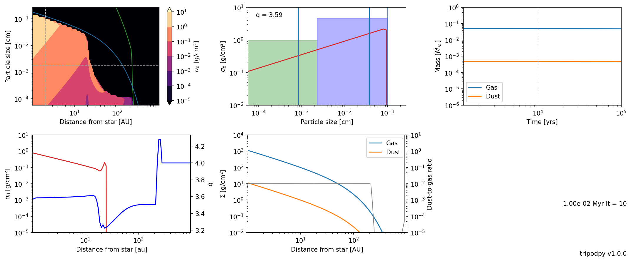
plot.panel(sim,show_limits=True,ir=20)
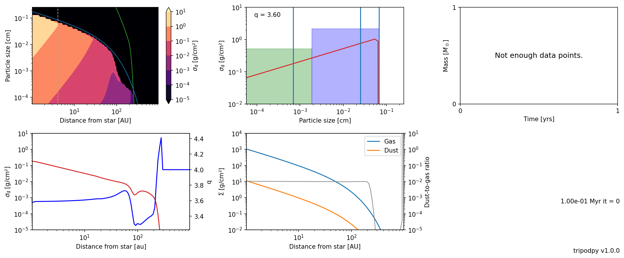
The blue and the green lines in the top left panel are analytical estimates for the fragmentation and drift barrier taken from Birnstiel et al. (2012). The middle panel on the top shows the size distribution at the radial index ir. The top right shows the mass evolution of dust and gas (if multiple snapshots are provided). The bottom left shows the midplane density of the dust (red) and the power law exponent q aka. \(\xi\) (blue). The
bottom middle pannel shows the total dust and gas surface desity along with the dust do gas ratio (gray) as a function of radius. If we pass the data directory as argument, we also have access to the time evolution. Furthermore, some plots can be adjusted by specifying the time it, radial ir, or size ia index.
[17]:
plot.panel("data", it=10, ir=10, ia=20)
Dust distribution with TriPoD
TriPoDPysimulates the evolution of the dust surface density in terms of the two population surface densities \(\Sigma_0\) and \(\Sigma_1\).
Together, they constitute the total dust density \(\Sigma_{tot} = \int \limits_{m\left(s_{min}\right)}^{m\left(s_{max}\right)} \sigma\left(m\right) \mathrm{d}m = \int \limits_{m\left(s_{min}\right)}^{m\left(s_{int}\right)} \sigma\left(m\right) \mathrm{d}m + \int \limits_{m\left(s_{int}\right)}^{m\left(s_{max}\right)} \sigma\left(m\right) \mathrm{d}m = \Sigma_0 + \Sigma_1\).
[18]:
SigmaTot = sim.dust.Sigma.sum(-1)
SigmaTot
[18]:
[1.11816465e+01 1.04183445e+01 9.70477551e+00 9.03822292e+00
 8.41623126e+00 7.83595545e+00 7.29466546e+00 6.78979477e+00
 6.31893572e+00 5.87983130e+00 5.47036721e+00 5.08856402e+00
 4.73256977e+00 4.40065277e+00 4.09119469e+00 3.80268401e+00
 3.53370963e+00 3.28295483e+00 3.04919145e+00 2.83127432e+00
 2.62813594e+00 2.43878143e+00 2.26228369e+00 2.09777883e+00
 1.94446187e+00 1.80158268e+00 1.66844213e+00 1.54438864e+00
 1.42881484e+00 1.32115458e+00 1.22088020e+00 1.12750002e+00
 1.04055614e+00 9.59622497e-01 8.84303228e-01 8.14231318e-01
 7.49067575e-01 6.88499863e-01 6.32242471e-01 5.80034566e-01
 5.31629104e-01 4.86701769e-01 4.44833737e-01 4.05750353e-01
 3.69280669e-01 3.35434352e-01 3.04187869e-01 2.75371203e-01
 2.48806414e-01 2.24327155e-01 2.01785224e-01 1.81051909e-01
 1.62016500e-01 1.44574390e-01 1.28627518e-01 1.14080000e-01
 1.00834994e-01 8.87948903e-02 7.78657906e-02 6.79631535e-02
 5.90140081e-02 5.09564151e-02 4.37432311e-02 3.73549731e-02
 3.17840475e-02 2.69552356e-02 2.27335733e-02 1.90178477e-02
 1.57507053e-02 1.29151878e-02 1.04876296e-02 8.43199312e-03
 6.70878990e-03 5.27902614e-03 4.10241710e-03 3.12740682e-03
 2.26042366e-03 1.35092232e-03 4.32536686e-04 7.90011850e-05
 9.09758036e-06 7.01977289e-07 2.00000000e-11 2.00000000e-11
 2.00000000e-11 2.00000000e-11 2.00000000e-11 2.00000000e-11
 2.00000000e-11 2.00000000e-11 2.00000000e-11 2.00000000e-11
 2.00000000e-11 2.00000000e-11 2.00000000e-11 2.00000000e-11
 2.00000000e-11 2.00000000e-11 2.00000000e-11 2.00000000e-11]
In order to display the data in a more granular way and compare it to Dustpy outputs, we can use the distribution exponents \(\xi\) to interpolate the dust surface density over a logarithmic mass grid. The density in the mass interval \(\left[m_0, m_1\right]\) is then given by
\(\Sigma_{[m_0, m_1]} = \int\limits_{m_0}^{m_1} \sigma\left(m\right) \mathrm{d}m = \Sigma_{tot} \frac{m_1^{\frac{\xi+4}{3}}-m_0^{\frac{\xi+4}{3}}}{m_{max}^{\frac{\xi+4}{3}}-m_{min}^{\frac{\xi+4}{3}}}\) for \(\xi_{calc} \neq -4\) and \(\Sigma_{tot} \frac{\log(m_1/m_0)}{\log(m_{max}/m_{min})}\) for \(\xi_{calc} = -4\).
This calculation is automatically done in the data readout scheme of the plotting routine:
[19]:
from tripodpy.utils import read_data
data = read_data("data")
The plotted dust density distribution is then given by
\(\Sigma_\mathrm{d} = \int\limits_0^\infty \sigma \left(m \right) \mathrm{d} \log m\).
In this way the distribution is independent of the mass grid.
The internal dust distribution TriPoDPy uses after interpolation of the dust density are \(\Sigma_{\mathrm{d},\,i} \equiv \Sigma_\mathrm{d} \left(m_i \right)\) with
\(\Sigma_\mathrm{d} = \sum\limits_i \Sigma_{\mathrm{d},\,i}\),
meaning the numerical sum over the mass dimension is the dust surface density.
[20]:
data.dust.Sigma_recon.sum(-1)[-1,...]
[20]:
array([1.11816465e+01, 1.04183445e+01, 9.70477551e+00, 9.03822292e+00,
       8.41623126e+00, 7.83595545e+00, 7.29466546e+00, 6.78979477e+00,
       6.31893572e+00, 5.87983130e+00, 5.47036721e+00, 5.08856402e+00,
       4.73256977e+00, 4.40065277e+00, 4.09119469e+00, 3.80268401e+00,
       3.53370963e+00, 3.28295483e+00, 3.04919145e+00, 2.83127432e+00,
       2.62813594e+00, 2.43878143e+00, 2.26228369e+00, 2.09777883e+00,
       1.94446187e+00, 1.80158268e+00, 1.66844213e+00, 1.54438864e+00,
       1.42881484e+00, 1.32115458e+00, 1.22088020e+00, 1.12750002e+00,
       1.04055614e+00, 9.59622497e-01, 8.84303228e-01, 8.14231318e-01,
       7.49067575e-01, 6.88499863e-01, 6.32242471e-01, 5.80034566e-01,
       5.31629104e-01, 4.86701769e-01, 4.44833737e-01, 4.05750353e-01,
       3.69280669e-01, 3.35434352e-01, 3.04187869e-01, 2.75371203e-01,
       2.48806414e-01, 2.24327155e-01, 2.01785224e-01, 1.81051909e-01,
       1.62016500e-01, 1.44574390e-01, 1.28627518e-01, 1.14080000e-01,
       1.00834994e-01, 8.87948903e-02, 7.78657906e-02, 6.79631535e-02,
       5.90140081e-02, 5.09564151e-02, 4.37432311e-02, 3.73549731e-02,
       3.17840475e-02, 2.69552356e-02, 2.27335733e-02, 1.90178477e-02,
       1.57507053e-02, 1.29151878e-02, 1.04876296e-02, 8.43199312e-03,
       6.70878990e-03, 5.27902614e-03, 4.10241710e-03, 3.12740682e-03,
       2.26042366e-03, 1.35092232e-03, 4.32536686e-04, 7.90011850e-05,
       9.09758036e-06, 7.01977289e-07, 2.00000000e-11, 2.00000000e-11,
       2.00000000e-11, 2.00000000e-11, 2.00000000e-11, 2.00000000e-11,
       2.00000000e-11, 2.00000000e-11, 2.00000000e-11, 2.00000000e-11,
       2.00000000e-11, 2.00000000e-11, 2.00000000e-11, 2.00000000e-11,
       2.00000000e-11, 2.00000000e-11, 2.00000000e-11, 2.00000000e-11])
For a more in depth analysis the internally used sizes and power law exponents can be found in the simulation Object/data under:
power law exponent of the particle size distribution:
[21]:
sim.dust.qrec[:5]
[21]:
[-3.57885522 -3.58436399 -3.58985937 -3.59026723 -3.59045478]
the minimum and maximum sizes of the distribution:
[22]:
sim.dust.s.min[:5]
[22]:
[5.22875516e-05 5.22875516e-05 5.22875516e-05 5.22875516e-05
 5.22875516e-05]
[23]:
sim.dust.s.max[:5]
[23]:
[0.13647524 0.13476168 0.13092258 0.12635921 0.12193889]
the size array with all the sizes used for the evolution of the distribution:
\([a_0, 0.4 * a_1, a_1, 0.4 * a_{max}, a_{max}]\)
[24]:
sim.dust.a[0,:]
[24]:
[0.00097461 0.01991676 0.04979191 0.0545901 0.13647524]
this means all the dust quantities either have shape \((N_r, 2)\) or \((N_r, 5)\) depending if they are defined for the mass bins or the particle sizes
Reading data files
If we want to read data files, we can use the read/writer module provided by simframe that is used to write the data.
[25]:
from dustpy import hdf5writer

wrtr = hdf5writer()
We should make sure that the correct data directory is assigned to the writer.
[26]:
wrtr
[26]:
Writer (HDF5 file format using h5py)
------------------------------------
    Data directory : data
    File names     : data/data0000.hdf5
    Overwrite      : False
    Dumping        : True
    Options        : {'com': 'lzf', 'comopts': None}
    Verbosity      : 1
We can now read a single data file with
[27]:
data0003 = wrtr.read.output(3)
This function returns a namespace and the data can simply be accessed in the same way as for the Simulation object.
[28]:
data0003.gas.Sigma
[28]:
array([1.11399371e+003, 1.03936331e+003, 9.69418292e+002, 9.03901717e+002,
       8.42577816e+002, 7.85223246e+002, 7.31620090e+002, 6.81552405e+002,
       6.34806398e+002, 5.91172929e+002, 5.50450541e+002, 5.12447758e+002,
       4.76984260e+002, 4.43891110e+002, 4.13010428e+002, 3.84194816e+002,
       3.57306712e+002, 3.32217749e+002, 3.08808143e+002, 2.86966128e+002,
       2.66587413e+002, 2.47574692e+002, 2.29837176e+002, 2.13290157e+002,
       1.97854607e+002, 1.83456798e+002, 1.70027947e+002, 1.57503892e+002,
       1.45824781e+002, 1.34934785e+002, 1.24781832e+002, 1.15317357e+002,
       1.06496066e+002, 9.82757223e+001, 9.06169385e+001, 8.34829889e+001,
       7.68396309e+001, 7.06549389e+001, 6.48991486e+001, 5.95445117e+001,
       5.45651595e+001, 4.99369755e+001, 4.56374756e+001, 4.16456957e+001,
       3.79420864e+001, 3.45084138e+001, 3.13276659e+001, 2.83839651e+001,
       2.56624852e+001, 2.31493726e+001, 2.08316729e+001, 1.86972608e+001,
       1.67347738e+001, 1.49335495e+001, 1.32835669e+001, 1.17753902e+001,
       1.04001165e+001, 9.14932670e+000, 8.01503936e+000, 6.98966853e+000,
       6.06598484e+000, 5.23708046e+000, 4.49633800e+000, 3.83740365e+000,
       3.25416470e+000, 2.74073163e+000, 2.29142506e+000, 1.90076741e+000,
       1.56347942e+000, 1.27448129e+000, 1.02889813e+000, 8.22069157e-001,
       6.49560116e-001, 5.07177865e-001, 3.90986192e-001, 2.97321654e-001,
       2.22808174e-001, 1.64369134e-001, 1.19235769e-001, 8.49508478e-002,
       5.93668651e-002, 4.06383541e-002, 2.72082855e-002, 1.77889719e-002,
       1.13382867e-002, 7.03235028e-003, 4.23606956e-003, 2.47302040e-003,
       1.39611750e-003, 7.60333317e-004, 3.98435021e-004, 2.00348591e-004,
       9.63848531e-005, 4.42233694e-005, 1.92860885e-005, 7.96543382e-006,
       3.10355024e-006, 1.13600681e-006, 3.87860290e-007, 1.00000000e-100])
We can also read the entire data directory with
[29]:
data = wrtr.read.all()
The data has now an additional dimension for time.
[30]:
data.gas.Sigma.shape
[30]:
(21, 100)
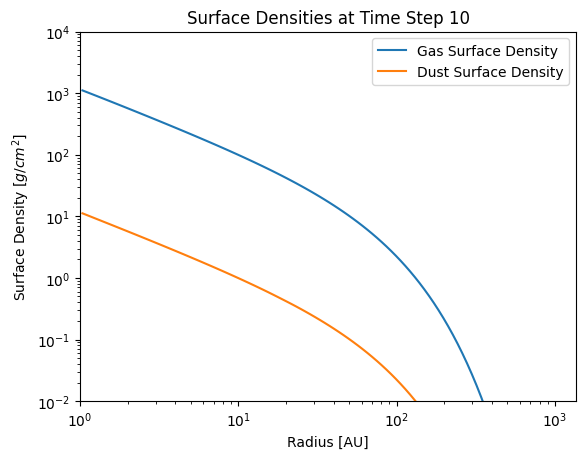
the simulation data can also be comfortably plotted from the data read, for example we can reproduce the last plot form the panel function as follows:
[31]:
import matplotlib.pyplot as plt
[32]:
# Time step we want to plot
it = 10
plt.figure()
plt.plot(data.grid.r[it,:]/c.au, data.gas.Sigma[it, :], label='Gas Surface Density')
#total dust surface density
plt.plot(data.grid.r[it,:]/c.au, data.dust.Sigma[it,...].sum(-1), label='Dust Surface Density')
plt.xlabel('Radius [AU]')
plt.ylabel('Surface Density $[g/cm^2]$')
plt.title(f'Surface Densities at Time Step {it}')
plt.xscale('log')
plt.yscale('log')
plt.ylim(1e-2, 1e4)
plt.xlim(1)
plt.legend()
plt.show()
Data files can be quite large and reading the entire data set can consequently take some time. Instead, it is more efficient to only read single fields from the data files. We can do so via e.g.
[33]:
SigmaGas = wrtr.read.sequence("gas.Sigma")
[34]:
SigmaGas.shape
[34]:
(21, 100)
It is also possible to exclude certain fields from being written into the data files to save memory by setting their save attribute to False.
[35]:
sim.dust.v.save = False
Reading Dump Files
The data files merely contain the pure data, but no information about the operations TriPoDPy has to perform, e.g. customized functions. Hence, it is not possible to directly restart a simulation from data files.
simframe is saving by default the most recent dump file, from which a simulation can be restarted.
Attention: Malware can be injected with dump files, which are pickled objects. One should only read dump files that were created by oneself or from trusted sources! Dump files have to be read with the same version of TriPoDPy as they were written. Otherwise, it is not guaranteed to work.
[36]:
from dustpy import readdump
[37]:
sim_restart = readdump("data/frame.dmp")
This is now a simulation frame that should be identical to our previous object.
[38]:
sim.gas.Sigma == sim_restart.gas.Sigma
[38]:
[ True  True  True  True  True  True  True  True  True  True  True  True
  True  True  True  True  True  True  True  True  True  True  True  True
  True  True  True  True  True  True  True  True  True  True  True  True
  True  True  True  True  True  True  True  True  True  True  True  True
  True  True  True  True  True  True  True  True  True  True  True  True
  True  True  True  True  True  True  True  True  True  True  True  True
  True  True  True  True  True  True  True  True  True  True  True  True
  True  True  True  True  True  True  True  True  True  True  True  True
  True  True  True  True]
We can now, for example, add more snapshots and restart the simulation. Here we just want to extend the run by one year.
[39]:
from dustpy import constants as c

sim_restart.t.snapshots = np.concatenate((sim_restart.t.snapshots, [100001.*c.year]))
The current time is
[40]:
sim_restart.t / c.year
[40]:
100000.0
We can now restart the simulation for another year after the time of the dumpfile (which is automatically used).
[41]:
sim_restart.run()
tripodpy v1.0.0

Writing file data/data0021.hdf5
Writing dump file data/frame.dmp
Execution time: 0:00:00
Another file was written and the current time is now
[42]:
sim_restart.t / c.year
[42]:
100001.0